 AM modulation, illustrated
AM modulation, illustrated
AM modulation, illustrated
Radio is the one thing I'd like to play with, but I have not. For several reasons, this interest of mine always end up buried deep at in-tray, and perhaps I'll never fiddle with it, after all.
For a signal to travel over radio waves, it must be modulated first, which means having it transposed to a frequency bandwidth and format suitable to the transmission medium. Modulation techniques are closely related to telecommunications and information theory, and it is possible to play with modulation within the limits of a computer. This is a theme that I must confess I don't understand much, but I am mesmerized by it nevertheless. And to be honest, I find incredible how a couple simple calculations can make the miracle.
In this post, I am going to illustrate the AM modulation techniques, using WAV audio files. To begin with, we need a baseband signal, that is, some audio that fills all available bandwidth from 0Hz. I have recorded my own, ugly voice in order to torture your ears:
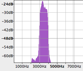
The bandwidth or frequency spectrum of this speech is:
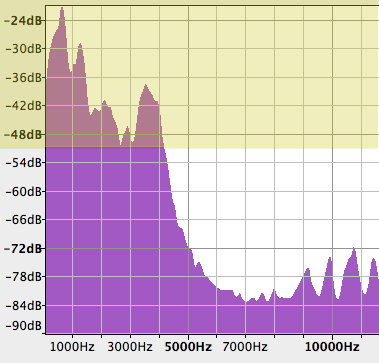
The yellow part of the spectrum is the relevant one, since the Y axis is logarithmic (dB). 20 decibels means a difference of 100 times, so the spectrum contents above 5000Hz is mostly "digital noise", not actual content. In the next graphs I will crop out the bottom of the graph. (If you are curious or don't trust my graphs, you can always download the WAV files and look into their spectrum yourself.)
AM modulation demands that signal is restricted to a bandwidth, so the modulated signal will also "fit" in a predetermined frequency band. So, we need to apply a low-pass filter on my voice, and we define the cut-off at 1000Hz. The result is my voice in lower quality.
The spectrum of this filtered signal is:
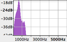
I have used an Audacity's low-pass filter plug-in, which is not perfect but it is enough to illustrate our points. In other posts, I write a filter from scratch, in Python.
Amplitude modulation is just the product of the original signal by the carrier, a sinusoidal wave. In this case, I have chosen a 3000Hz carrier, well above the cut-off of original signal, which is 1000Hz. The carrier noise itself is:
Modulation result (voice multiplied by whistle) is:
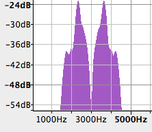
Note that it is almost impossible to understand the speech. To be exact, this modulation is named AM-SC (Supressed Carrier), for a reason that I will clarify a bit later.
Modulation makes my voice to exchange band from 0-1000 to 2000-4000Hz. Actually, AM modulation creates two "copies" of the original signal, one at 2000-3000Hz band and another at 3000-4000Hz. So, normal AM "wastes" bandwidth because modulated signal occupies twice as much of bandwidth:
Nevertheless, AM-SC is still quite useful, because I can "move" my voice to frequencies suitable for electromagnetic transmission. And, even more important, modulation allows allocation of multiple signals on the same medium, each one occupying a different band, and each one can be recovered separately.
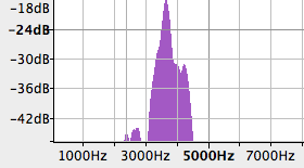
The "normal", broadcasting AM radio modulation sounds like this:
In this modulation, we can hear the carrier, while we could not in AM-SC. The spectrum is similar to AM-SC but it has an additional sharp "spike" at carrier frequency:

The following Python program was employed to generate the modulated AM and AM-SC audios:
#!/usr/bin/env python

import wave, struct, math

baseband = wave.open("paralelepipedo_lopass.wav", "r")

amsc = wave.open("amsc.wav", "w")
am = wave.open("am.wav", "w")
carrier = wave.open("carrier3000.wav", "w")

for f in [am, amsc, carrier]:
    f.setnchannels(1)
    f.setsampwidth(2)
    f.setframerate(44100)

for n in range(0, baseband.getnframes()):
    base = struct.unpack('h', baseband.readframes(1))[0] / 32768.0
    carrier_sample = math.cos(3000.0 * (n / 44100.0) * math.pi * 2)

    signal_am = signal_amsc = base * carrier_sample
    signal_am += carrier_sample
    signal_am /= 2

    amsc.writeframes(struct.pack('h', signal_amsc * 32767))
    am.writeframes(struct.pack('h', signal_am * 32767))
    carrier.writeframes(struct.pack('h', carrier_sample * 32767))
AM-SC is simply the original (ifbandwidth-restricted) signal multiplied by the carrier, which is simply a sinusoidal wave.
AM modulation is the same as AM-SC, except the carrier is added afterwards. This allows the AM receiver to be much simpler, as we will see.
Well, it's time to prove we can extract the original voice from these modulated audios. The AM-SC demodulation is basically the same as modulation: multiply by a carrier sinusoid.
These are the demodulated audios, first without lowpass filtering:
And with lowpass filtering:
For those who prefer to see the modulation happening in time domain, the following figure shows the waveforms of AM-SC. Blue is the original signal, red is the carrier, purple is the modulated signal, and green is unfiltered demodulated signal on receiver.
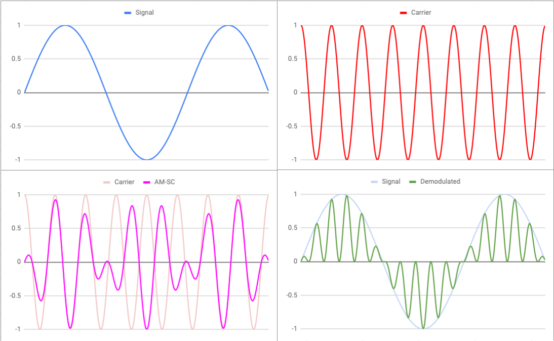
Note the AM-SC modulated signal shows a "wrapper" or envelope, that is, the wave peaks bear a relationship with the original (blue) signal, as if they were wrapped by the signal.
Multiplying a signal twice by the same carrier throws the voice back to its original band (0-1000Hz), and creates a new copy around 6000Hz which needs to be supressed by the lowpass filter.
This is the AM-SC demodulator code:
modulated = wave.open("amsc.wav", "r")

demod_amsc_ok = wave.open("demod_amsc_ok.wav", "w")
demod_amsc_nok = wave.open("demod_amsc_nok.wav", "w")
demod_amsc_nok2 = wave.open("demod_amsc_nok2.wav", "w")

for f in [demod_amsc_ok, demod_amsc_nok, demod_amsc_nok2]:
    f.setnchannels(1)
    f.setsampwidth(2)
    f.setframerate(44100)

for n in range(0, modulated.getnframes()):
    signal = struct.unpack('h', modulated.readframes(1))[0] / 32768.0
    carrier = math.cos(3000.0 * (n / 44100.0) * math.pi * 2)
    carrier_phased = math.sin(3000.0 * (n / 44100.0) * math.pi * 2)
    carrier_freq = math.cos(3100.0 * (n / 44100.0) * math.pi * 2)

    base = signal * carrier
    base_nok = signal * carrier_phased
    base_nok2 = signal * carrier_freq

    demod_amsc_ok.writeframes(struct.pack('h', base * 32767))
    demod_amsc_nok.writeframes(struct.pack('h', base_nok * 32767))
    demod_amsc_nok2.writeframes(struct.pack('h', base_nok2 * 32767))
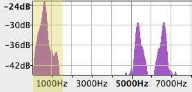
The new copy of the information at 6000Hz, that I call "demodulation noise", is puzzling to some readers. They simulate things in a spreadsheet and don't understand why such a high-frequency component is there.
Here is the spectrum of the demodulated AM-SC audio, before the necessary low-pass filtering. The yellow part is the "good" part:
It is interesting to use a bit of math to clarify this point. This applies for AM and QAM as well. The original audio information f(t) is modulated (multiplied) by a cosine wave, the carrier. So the transmitted signal is f(t).cos(t). Demodulation transforms it into f(t).cos(t).cos(t). If we remember the high-school trigonometric identities, we can convert the last form into f(t).[1+cos(2t)] and to f(t)+[f(t).cos(2t)].
Now it is clear (if you are comfortable with formulas) that the demodulated signal is a sum of two parts: the decoded f(t) audio (that we want) and audio "modulated" at 2t (that we don't want). Since the carrier's frequency is much higher than the audio's bandwidth, the unwanted part falls on a high frequency band, eliminated by the crudest low-pass filter.
The little big problem of AM-SC demodulation is: the demodulator carrier must be EXACTLY equal to transmitter's, both in frequency and phase. Any difference will wreck the demodulation. In the code above, I simulated two demodulation problems: carrier with wrong phase (90 degrees behind), and with wrong frequency (100Hz higher). The results are very bad, as you can hear below (already lowpassed):
To be fair, the carrier can still recover the signal if the phase error is not exactly 90 degress, albeit with lower volume (the less the phase error, the higher the volume). So we can use a quadrature (I/Q) demodulator that uses two carriers delayed by 90º to detect the signal; the combination of their results will be the full-volume signal. But the carriers' frequency must still be exact.
AM-SC sends no hard reference of the carrier, and this limits the usage of AM-SC in real-world. AM is the most often used variant. (*)
Now, let's see the AM demodulator, actually an "envelope detector":
modulated = wave.open("am.wav", "r")

f = demod_am = wave.open("demod_am.wav", "w")
f.setnchannels(1)
f.setsampwidth(2)
f.setframerate(44100)

for n in range(0, modulated.getnframes()):
    signal = struct.unpack('h', modulated.readframes(1))[0] / 32768.0
    signal = abs(signal)
    demod_am.writeframes(struct.pack('h', signal * 32767))
Appreciate how simple it is; note the absence of transcendental functions. AM can be detected by a simple diode, which cuts off the negative part of wave. The diode can even be improvised with a galena crystal or a rusty razor blade.
This is the recovered audio after detection:
Low-pass filtered:
The remaining noise is due to the abs() detector, which creates "kinks" in the demodulated waveform. In a real-world AM radio, this noise would be of very high frequency, and easily removable. (Remember our carrier is just 3000Hz in these examples.)
Wave forms (time domain) in AM modulation:
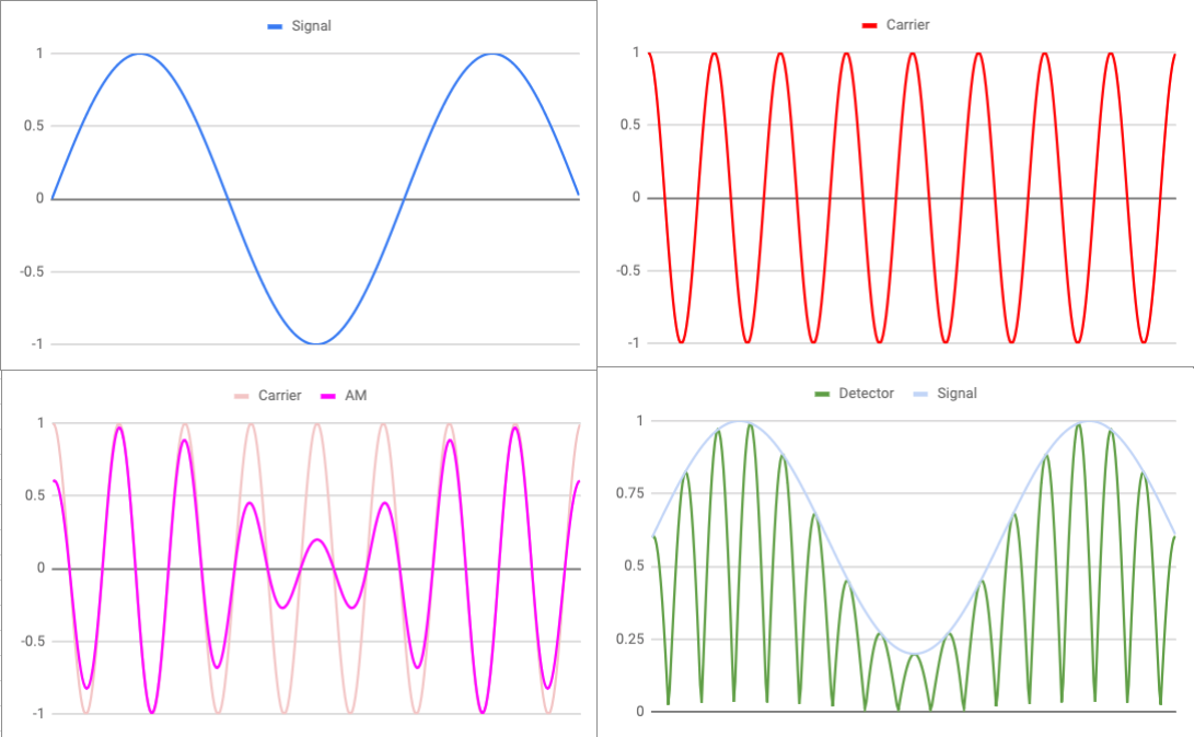
The modulated AM signal shows a stronger "envelope effect" than AM-SC: the wave peaks clearly follow the contour of the original signal, and that's why it is so easy to demodulate, it can happen even accidentally through dental obturations and other objects. (See this video if you don't believe me.)
By the way, the spreadsheet that generated the waveforms above can be opened here.
An AM receiver is not forced to use an envelope detector. The product detector also works and even has some advantages over a detector: improved noise resistance and compatibility with AM-SC and AM-SSB signals. It is easy to generate the carrier because AM sends it along with the payload.
AM is equivalent to AM-SC coupled with large DC bias to the signal. The bias guarantees the carrier is always multiplied by a positive value, and therefore the output is always in phase with the carrier. The AM signal phase does not carry any useful information, and the receiver just disregards it.
In AM-SC, the original content is modulated "as is". Negative signals inverts the carrier. The AM-SC result carries a bit of information in its phase: the polarity of the signal.
If you try to demodulate AM-SC with an envelope detector, the polarity information are lost. The result will be very off, even though it might resemble the original audio. If it was human voice, it will sound like Donald Duck, because the wrongful demodulation doubles the frequency and adds harmonics.
AM-SC has some advantages over AM. It is more efficient in bandwidth and power. Also, AM demodulation may lose some low-frequency signals, because the DC bias needs to be removed somehow, and the very low-frequency is discarded altogether. AM-SC can send content down to 0Hz. This is important for video signals.
Both AM and AM-SC modulations waste bandwidth, because they send two "copies" of the same content around the carrier. The AM also sends the carrier. An AM transmitter spends 75% of power sending excess information, just to nanny AM receivers.
Since the AM-SC signal has two copies, we can just filter out one of them, sending only the other. This is called AM-SSB (supressed side band). The spectrum will be obviously different from AM-SC, the sideband below 3000Hz is almost absent:
The SSB wave forms can be seen below:
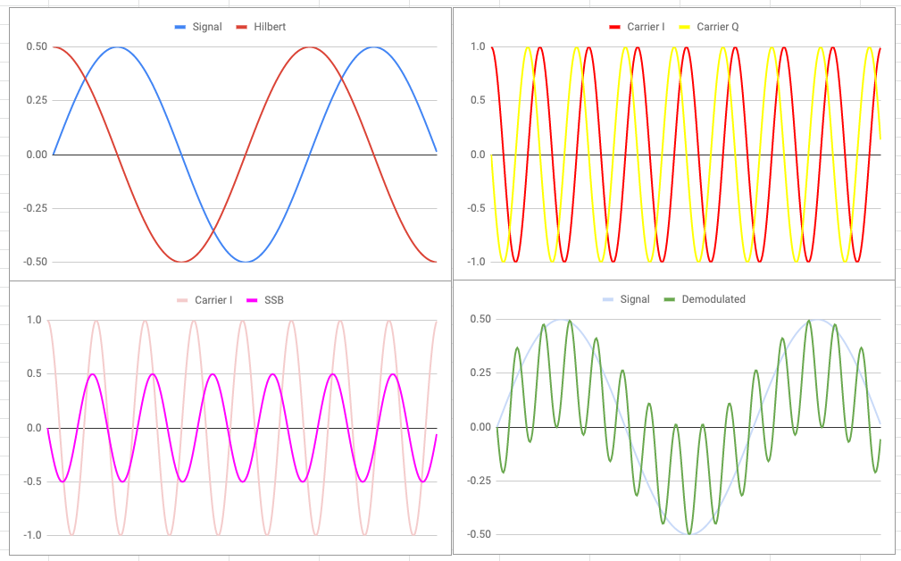
In the figure above, we have two new elements that you can ignore for now: a 'Hilbert' version of the signal, in red (and 90 degrees ahead); and a second 'Carrier Q' in yellow, also ahead of the original carrier. They will make sense later, when we talk about the Hilbert Transform.
Quite different from AM and AM-SC, the SSB modulated signal has no envelope, even though its amplitude is still proportional to the general amplitude of the original signal (0.5 in the figure). Since the original signal is a "pure" cosine, the modulated wave is also "pure", with frequency almost equal to the carrier. This is congruent with the fact that SSB is a perfect translation in frequency domain, with no additional copies nor distortions.
This is how AM-SSB sounds like (lower band removed, only upper band is kept):
Not much different from AM-SC; and in fact the AM-SC demodulator can cope with AM-SSB signal without any changes:
Low-pass filtered:
By sending only one copy of original content, and no carrier, AM-SSB saves bandwidth and power. It has a second big advantage over AM-SC. See what happens when we demodulate AM-SSB with an out-of-phase carrier:
The voice has been recovered perfectly. So, an AM-SSB receiver does not need to worry with carrier's phase. Only the demodulator frequency is important, and it must be watched closely; any frequency deviation causes audio distortion pretty much like AM-SC:
AM-SSB is the standard modulation for long-distance ham radio, analog TV video, etc. The same technique is employed in FDM multiplexers and countless other devices that need to fit many signals into a single channel.
SSB, like AM, can't transmit signals of very low frequency. Analog TV needs low-freq to be preserved, so it uses a variant named VSB (Vestigial Sideband). In VSB, a slice of the "other" sideband is kept, so the low-frequency content is demodulated as AM-SC, with a smooth transition to AM-SSB for higher frequencies.
The unwanted sideband can be removed by filters, but there are techniques to generate AM-SSB directly.
One interesting technique, employed by radios that are capable of DSP, is the Hilbert Transform. This transform changes the audio phase by 90 degrees. It is not simple delay; it is a phase change on every frequency present in the signal.
The Hilbert-transformed audio sounds the same because we can't hear phase differences. But, thanks to trigonometric identities, modulating this transformed signal with a phased carrier and adding it to AM-SC cancels out the lower-band "copy", leaving the upper-band. We get a perfect AM-SSB signal without any filtering.
The Hilbert Transform is most easily described and implemented in frequency domain (Fast Fourier Transform), but it can also be implemented as a FIR filter (convolution in time domain). Such filter will be "noncausal" (that is, depends on "future" samples), in practice this means that the filter yields a time-delayed result. It is easy to compensate for this, but it must not be forgotten.
The following Python script implements an AM-SSB modulator and implements Hilbert as a FIR filter.
#!/usr/bin/env python

import wave, struct, math, numpy

hlen = 500.0

hilbert_impulse = [ (1.0 / (math.pi * t / hlen)) \
			for t in range(int(-hlen), 0) ]
hilbert_impulse.extend([0])
hilbert_impulse.extend( [ (1.0 / (math.pi * t / hlen)) \
			for t in range(1, int(hlen+1)) ] )

hilbert_impulse = [ x * 1.0 / hlen for x in hilbert_impulse ]

baseband = wave.open("amssb_hilbert_orig.wav", "r")
amssbh = wave.open("amssb_hilbert.wav", "w")

for f in [amssbh]:
    f.setnchannels(1)
    f.setsampwidth(2)
    f.setframerate(44100)

base = []
base.extend([ struct.unpack('h',
                baseband.readframes(1))[0] / 32768.0 \
		for n in range(0, baseband.getnframes()) ])
base.extend([ 0 for n in range(0, int(hlen)) ])

base_hilbert = numpy.convolve(base[:], hilbert_impulse)

for n in range(0, len(base) - int(hlen)):
    carrier_cos = math.cos(3000.0 * (n / 44100.0) * math.pi * 2)
    carrier_sin = -math.sin(3000.0 * (n / 44100.0) * math.pi * 2)

    s1 = base[n] * carrier_cos
    # time-shifted signal because Hilbert transform is noncausal
    s2 = base_hilbert[n + int(hlen)] * carrier_sin

    signal_amssbh = s1 + s2

    amssbh.writeframes(struct.pack('h', signal_amssbh * 32767))
The spectrum analysis shows the lower (unwanted) sideband was more effectively wiped out by this technique than by simple filtering:
Generating an AM-SSB signal like this, with two phased carriers, suggests that AM-SSB is actually a special case of analog QAM (Quadrature Amplitude Modulation). QAM allows to transmit two signals at the same time, and we are sending two signals: the original audio and the Hilbert-transformed audio.
Both signals are interdependent and equivalent in information content, so we are, in a sense, sending two copies of the same thing — even though the intention is the removal of a sideband, not redundancy. The QAM phase angle is not fixed, it rotates all the time (and measuring the speed of this rotation would be a way to recover the original information).
Viewing AM-SSB as QAM also explains why the AM-SSB demodulator can always detect the original audio, even if the carrier is out of phase with the transmitter. Since the same audio is being sent twice, over two orthogonal carriers, the demodulator can always find one or another — or, most likely, a mix of both.
(*) FM stereo uses AM-SC. The second audio channel is encoded within the audio signal by a 38KHz carrier. A 19KHz pilot tone is sent along to synchronize the carrier.