 Diff algorithms
Diff algorithms
Diff algorithms
I guess that many readers have already used the diff command-line application, or have already seen a Git "patch" or "commit" whose contents are similar to this:
--- Analytics.java.old	2016-04-03 00:07:40.000000000 -0300
+++ Analytics.java	2016-04-03 00:07:50.000000000 -0300
@@ -78,15 +78,13 @@

         in_flight = true;

-        JsonObjectRequest req = new JsonObjectRequest(Request.POST,
+        JsonObjectRequest rez = new JsonObjectRequest(Request.GET,
                 new Response.Listener<JSONObject>() {
                     @Override
                     public void onResponse(JSONObject response) {
The file above is an edition script: a list of instructions that, once applied on the original file Analytics.java.old, makes it equal to the file Analytics.java. Apart from the gory details like the @@ and the magic numbers, it is easy to see that the script replaces a line ended in POST by another that ends in GET.
There are many "diff" formats around. The above format is the "Universal" format whose description can be found here. It is the most common these days. The widespread usage of Git promoted the Universal format even further. Many folks without Unix background have come to know the "diffs", by will or by force.
Since forever, I have been somewhat curious about the diff algorithm, but never looked into it, until I needed to implement something similar.
Explained: I have a set of unit tests. The test framework keeps an ongoing record of some critical states of the app. This data is captured along the execution of each unit test. It became important to detect behavior changes, even if the test passes. For example, during a test run, the states A,B,C,D,E are recorded. If another run observes a state sequence like A,D,C,B,E, there ought to be a good reason.
I needed an ergonomic tool that highlighted these differences. Generating two text files and comparing them with diff was not enough, and the concept "difference" must be flexible. For example, each record has timestamps that of course change in every run, but this should not trigger a difference. Wrapping up, I decided to implement a specific-purpose "diff".
If you just want an implementation of the best algorithm available, and does not want to know the inner workings, download and open this Zip, and look for the diff_myers.py script. It implements the Myers algorithm that is employed by every major application (diff, Git, etc.).
In the case of my app, the sensible thing to do would be to employ a ready-made module like this one. But "Man shall not live on bread alone"; reinventing the wheel is fun. I ended up with the following algorithm, laid out in Python-pseudocode:
# A and B are lists or strings to be compared

# Cut the "tail" (common trailing part)
while A and B and A[-1] == B[-1]:
	A.pop()
	B.pop()

while A or B:
	# Cut the "head" (common leading part)
	while A and B and A[0] == B[0]:
		A.pop(0)
		B.pop(0)

	minus = len(A)
	plus = len(B)
	cost = minus + plus

	# Find the next coincidence with least "cost"
	for i in range(0, len(A)):
		for j in range(0, len(B)):
			new_cost = i + j
			if new_cost > cost:
				break
			if A[i] == B[j]:
				if new_cost < cost:
					cost = new_cost
					minus = i
					plus = j
				break

	# Convert list slices into edition script
	edit("-", A[0:i])
	edit("+", B[0:j])
	A = A[i:]
	B = B[j:]
(A working implementation of this algorithm can be found here. The file within the Zip is diff_naive.py. This toy implementation compares two strings, passed as command-line parameters, but the core implementation is easily adaptable to any other purpose.)
The algorithm strategy is: cut the "head" (the leading parts of A and B that are equal); and then look for the next positions where a common element is found. Many common elements may be found, so it looks for the "least cost" one — that is, the element that can be reached with the minimal set of editions.
Strange as it seems, the algorithm works well, and I still use it in my unit test tool since it was good enough for this purpose.
Of course, the algorithm is far from optimal. First off, the execution time is O(mn). If A and B have 10k elements each, the processing could take up to 100M loop cycles. In practice it is not expected to happen, since A and B tend to similar and this spares the bulk of the potential effort. An advantage of this naïve algoritm is zero memory usage (apart from a handful of variables).
The biggest problem is the generation of sub-optimal scripts. "Sub-optimal" means that they are longer than strictly necessary. This is a use case that fooled the algorithm:
./diff_naive.py _C_D_E  _CD_E_
 _  C +D  _ -D +E  _ -E
The solution it found has 4 editions, but the optimal solution has only 2. Anyone can see that just moving one underscore is enough to convert _C_D_E to _CD_E_.
The naïve algorithm gets lost because there is a very common character: in this particular example, it is the underscore. They make plenty of "cheap" common elements between the strings under comparison. If we were comparing two source code files, the algorithm could be fooled by common lines like empty lines, close-bracket lines, etc.
This is a good example of "greedy" algorithm: it aims for short-term profits. There are cases that greedy algoritms are perfect, but not in this case.
On the other hand, the algorithm handles very well strings that have few repeated elements. For example, comparing ABCDE with BCDEXF is not a problem, since there is an intrinsic "order" among elements. Looking for C or for BCDE is the same, and looking for C alone is the smart thing to do, in this case.
In my use case, the "strings" are actually a list of machine states along the execution of a unit test. Every state is often unique within a given unit test. This explains why the algorithm worked well for me.
An easy modification is to "speculate" recursively what would be the total cost of the next algorithm steps, simulating the process until the end for every "branch". It kind of works, but it is extremely costly in terms of processing and stack, so it is not a real solution for general use.
It is also possible to design a (sub-optimal) diff algorithm around common substrings. The script diff_lcstr.py implements this idea using recursion. The pseudocode:
def lcstr(A, B):
	cut the leading common elements ("head")
	cut the trailing common elements ("tail")
	S = find the longest common substring in A and B

	if len(S) = 0:
		list A elements as "-" editions
		List B elements as "+" editions
		Finish

	lcstr(A[:A.indexOf(S)], B[:B.indexOf(S)])
	lcstr(A[A.indexOf(S)+len(S):], B[B.indexOf(S)+len(S):])
The algorithm above finds the longest common substring, discards it, and recursively handles the remaining slices of A and B, left and right of the substring, until no substring can be found.
At first glance, this algorithm seems to be smarter than the naïve version:
./diff_lcstr.py _C_D_E  _CD_E_
 _  C -_  D  _  E +_
But this algorithm can also be fooled, and sometimes it generates even worse results than the naïve version:
./diff_naive.py _C_D_EFGH_  _CD_E_F_G_H_
 _  C +D  _ -D +E  _ -E  F +_  G +_  H  _

/Users/epx $ ./diff_lcstr.py _C_D_EFGH_  _CD_E_F_G_H_
 _  C -_  D  _  E -F -G +_ +F +_ +G +_  H  _

/Users/epx $ ./diff_myers.py _C_D_EFGH_  _CD_E_F_G_H_
 _  C -_  D  _  E +_  F +_  G +_  H  _
In computer science, the 'best' edition script is the shortest possible. A good diff algorithm finds the shortest script, using CPU and memory sparingly.
There may be applications in which the "best" edition script, subjectively speaking, may not be the shortest one — in particular when a human is going to read the script. For example:
./diff_myers.py OBAMA BUSH
-O  B -A -M -A +U +S +H
The script above is "optimal" because it reuses the B letter, generating 7 editions instead of 9. But, subjectively speaking, it would be best to do -(OBAMA) +(BUSH), don't you agree? :)
By the way, Git implements Patience Diff, a variation of the diff algorithm that aims to generate human-friendly patches.
At this point, we will adopt the generally accepted definition: the best edition script is the shortest possible, and a good algorithm always finds it. The diff problem is equivalent to another computer science problem: find the longest common subsequence, known as LCS.
LCS is not the longest common substring; LCS allows to delete elements from both strings in order to find the longest string. For example, LCS("_C_D_E","_CD_E_") is equal to "_CDE". The longest common substring is "D_E". On the other hand, LCS("OBAMA","BUSH") is "U", and the longest common substring is also "U", in this case.
Once the LCS is found, all it takes is to recast the deletions into an edition script. The deletions on first string become "-", the deletions on second string become "+":
./diff_myers.py _C_D_E  _CD_E_
 _  C -_  D  _  E +_
For clarity, I will replace the underscores by "X", which does not change the spirit of the result:
./diff_myers.py xCxDxE  xCDxEx
 x  C -x  D  x  E +x
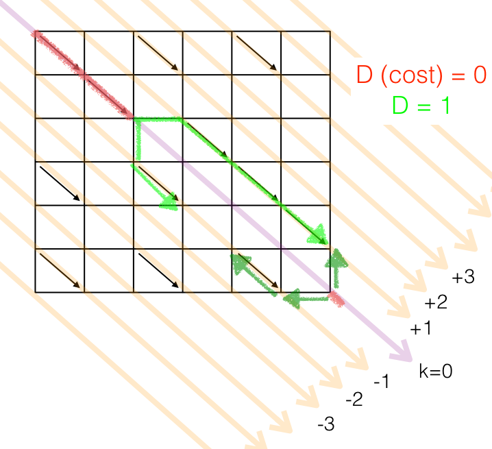
The LCS discovery process can be modeled as a graph:
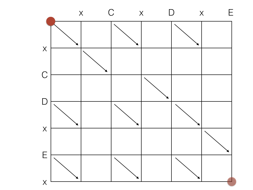
The objective of this "game" is move the red point from the upper left corner to the lower right corner, using as few straight moves as possible. The point can move left, right, or diagonally when there is a diagonal line available. The shortest path is the LCS.
The "length" of the path, that scientific articles name "D", and the naïve algorithm called "cost", is the sum of straight moves. In the figure above, the path has cost D=2. The diagonal moves don't count, so the shortest path is the one that contains as many diagonals as possible. Given strings A and B, the longest LCS path cannot be longer than len(A)+len(B).
The "old" string A is laid horizontally. The "new" string B is laid vertically. The diagonals represent elements in common between A and B. Every move to the right represents a deletion in string A (which will be interpreted as a deletion in the edition script). Every move down represents a deletion in string B (which will be interpreted as an insertion in the edition script).
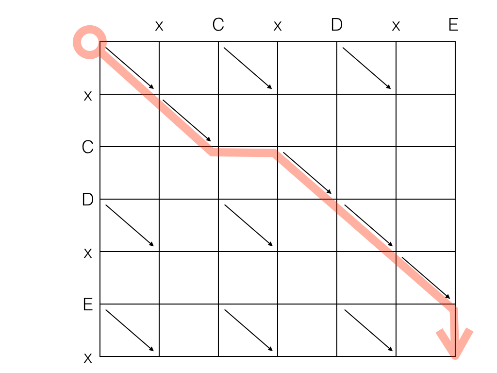
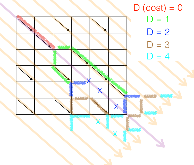
Now we can represent, and analyse, the "wrong" LCS found by the naïve algorithm:
Since this is a trivial example, bad luck was a factor: at point (2,2), the naïve algorithm elected to go down instead of to the right, even though the nearest diagonals were equally distant. The algorithm saw either option as equally good, but they were not. If we added characters to string A in the right place e.g. making it "xCx____DxE", the naïve algorithm will always go the wrong path, even in a lucky day.
With this graph, we can see clearly how the naïve algorithm works: it always looks for the nearest diagonal given its current location, without speculating about what comes next.
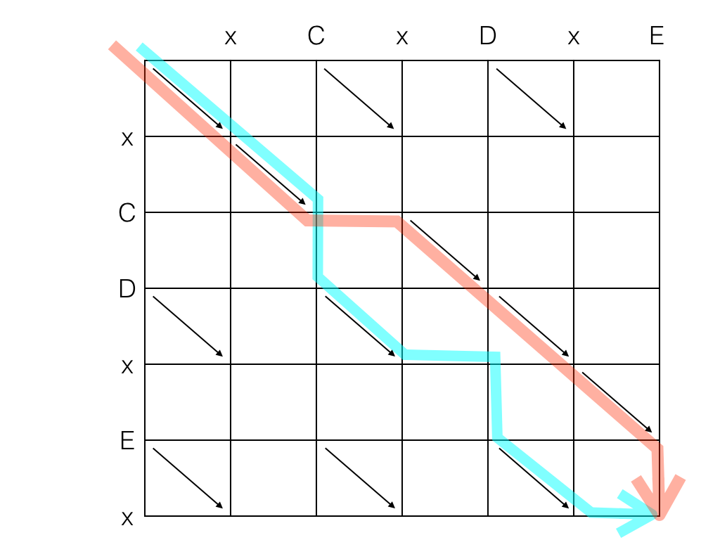
The substring-based algorithm always looks for the longest chain of diagonals. Sometimes this strategy works beautifully. But it misses badly if e.g. there is a small chain of diagonals in a corner, and many single diagonals scattered in the rest of the graph:
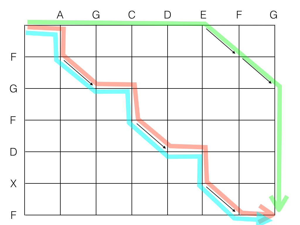
In the case above, the naïve algorithm followed the optimal path, because looking always for the nearest diagonal was incidentally the right thing to do. The same strings from figure above processed by our sample scripts:
./diff_lcstr.py AGCDEFG FGFDXF
Longest: FG
-A -G -C -D -E  F  G +F +D +X +F

./diff_myers.py AGCDEFG FGFDXF
-A +F  G -C +F  D -E +X  F -G
Even though the second edition script is shorter, the first one is actually more readable by a human being. Many folks would say that the first one is (subjectively) "better".
The best diff algorithm known to date is based on the fact that the count of long diagonals on an LCS graph grows linearly, not quadratically.

The literature names these long diagonals as k. They are numbered, beginning with the middle diagonal k=0 that starts at upper left corner. The diagonals above k=0 get positive numbers, negative otherwise. For an NxM graph, no more than M+N diagonals need to be considered.
The algorithm creates several paths that start small, but are extended, fed one straight movement at a time, until one path reaches the lower right edge. Obviously, the first worry is how to store all these paths in memory. The "wow" of the algorithm is that no more than M+N paths need to be tracked: one path per long diagonal.
The next Figure illustrates how the algorithm works:
The graph above is the same as xCxDxE/xCDxEx diff. The "step zero", in red, has zero cost because it simply skips leading common elements on both strings. There is only one path and it lies on k=0.
At step 1 (green), the algorithm spawns two paths, feeds each one with one straight move. One path went to long diagonal k=1, the other went to k=-1. Both paths found diagonals that allowed them to extend "for free".
At step 2 (dark blue), two paths become three. Note that two spaws go to k=0, but only the most promising survives. The other is killed (see the blue X's). At this point the algorithm can stop already, since one path reached the objective.
If the graph were larger, the extensions would go on accordingly to the brown segments (D=3) and clear blue (D=4). An aspect actively exploited by the algorithm is, a path with length D must have its 'front' on a long diagonal numbered (-D, -D+2, ..., D-2, D). So, at every cycle, the path fronts fill either even or odd diagonals.
The Eugene Myers' original article contains pseudocode, and explains how things work in a very precise and rigorous manner. If you compare the script diff_myers.py with the article, you will see how similar they are. The article is pretty amicable with developers in this regard, even though the rest of the text is dense.
A "problem" of Myers algoritm is that it only walks the optimal path and does not store it anywhere. Extracting the edition script from it, is an implementer's problem. In my implementation (diff_myers.py) I simply stow all intermediate points for every path, which is a bit wasteful, and the quadratic memory usage would be prohibitive in certain applications.
The Unix diff utility, and all its "spiritual descendants" like Git employ a clever strategy: they run the algorithm from both ends at the same time.
When two opposing paths meet, the latest sprout of either path is transformed into a piece of edition script. All implementations call this sprout "middle snake". The sub-graphs before and after the "middle" snake are recursively handled in the same fashion, finding two sub-snakes that generate two more pieces for the edition script, etc. until nothing is left.
This method has the big advantage of not needing memory to store whole paths. The edition script is composed as recursion advances. The payback is a modest usage of stack and twice as much processing.
An older algoritm that was once employed in Unix diff, is the Hunt-McIlroy. It is of historical interest. Also, it may look more intuitive than the Myers' algorithm. It generates good edition scripts, but not necessarily the optimal ones.
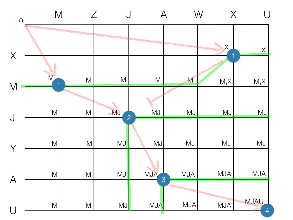
The "classic" LCS algorithm calculates a whole MxN matrix with the partial LCS lengths at every coordinate. Then it looks for the shortest path to connect the LCS length transitions. The figure above illustrates the process, showing the partial LCS at every point (M, MJ, MJA, MJAU).
The green lines are the "frontiers" where the LCS length changes. Note that each frontier effectively splits the graph in two regions, and one cannot go from e.g. from LCS=1 to LCS=3 without crossing the region LCS=2.
The main problem of the classic version is the usage of a big square of memory (MxN). This means 100M for a comparison of two 10k-element strings!
The Hunt-McIlroy algorithm focus exclusively on the so-called "k-candidates" — the blue balls where the two strings have common elements. (Making an array with all k-candidates, instead of MxN, is a big upfront reduction in memory usage.) These balls are important since that's where the partial LCS's change length. (After all, common subsequences can only exist if there are individual elements in common.)
In the typical case, the k-candidates will be few. Searching a path between them is efficient. A crucial rule of the algorithm is never going back (up or left). In the figure, the k-candidate near the right top corner is a dead-end, because the single Level-2 ball is at left of it, and it is forbidden to go left.
The solution found may be optimal or not, depending on the strategy of linking the k-candidates to find an end-to-end path. Simple strategies tend to measure only the distance from one k-candidate to the next, and will be suboptimal. On the other hand, an optimal solution (that explores all possible paths) tends to use too much memory.
This algorithm is a good example of "dynamic programming". This term means that the algorithm stores intermediate results in a memory table. In this case, the table contains k-candidates.