 Fundamental theorem of algebra
Fundamental theorem of algebra
Fundamental theorem of algebra
The polynomial equations are known since Antiquity, since they arise naturally from day-to-day questions. For example: if a rectangular plot of land has area 6 and semiperimeter 5 (perimeter 10), what are the dimensions of this plot?
This problem can be solved with a second-degree equation, that one you solve with Bhaskara, as everybody learns at school. The canonical form of the quadratic equation is
ax2 + bx + c = 0
Thanks to the Fundamental Theorem of Algebra, we know this equation has two roots, that is, two values of x that fulfill the equality. This allows to rewrite the equation in a different form, as a product of binomials:
a(x - x1)(x - x2) = 0
In this form, it is evident that coefficient a is just a scale factor that does not affect the values of the roots. So we can always multiply an equation by a constant to make a=1, making it equivalent to the form
(x - x1)(x - x2) = 0
If we multiply these binomials, we find the coefficients are symmetrical functions of the roots, i.e. they can be shuffled around. The coefficient b is simply the sum of the roots, the coefficient c is their product:
-b = x1 + x2
c = x1x2
These are the Viète formulas of the coefficients. By the way these formulas fit like a glove in our initial problem: if we consider the roots x1 and x2 as the sides of a rectangular land plot, then b is the semiperimeter (the negative of, actually), and c is the area.
Replacing the coefficients by the semiperimeter and the area, the equation becomes
x2 - 5x + 6 = 0
This particular equation is found throughout school textbooks since the solutions are integers. The roots, and the sides of the plot of land, are 2 and 3.
The Fundamental Theorem of Algebra (FTA) is a simple proposition: a polynomial equation of degree n and complex coefficients has at least one complex root.
Remember that rational numbers (Q) and real numbers (R) are inside the field of complex numbers (C). So, polynomials with real, rational or integer coefficients are even more guaranteed by the FTA to have roots.
Mathematicians believed the FAT was true long before it was proven. Proving it took a while, because the necessary mathematical tools were still being forged. Gauss finally proved it at the beginning of 19th century. Other proofs were found, and it continued to be subject of studies into the 20th century.
There is no purely algebraic proof, which is ironic. We can say FTA is a point of contact between algebra and other branches of math. The proof I will show is the same as described in this video, which was the first one that really "clicked" for me, as a non-mathematician.
The first thing one must understand to get this proof, is the difference of the graph of a complex function, when compared to an "ordinary" function. We are more accustomed with real-function graphs, where the independent variable is the X axis, and the function value lies in the Y axis.
For example, the figure below is a graph of our example equation, for real values of x:
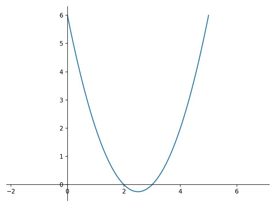
But how we can plot a graph, in a meaningful way, when x is complex, and y might be complex as well?
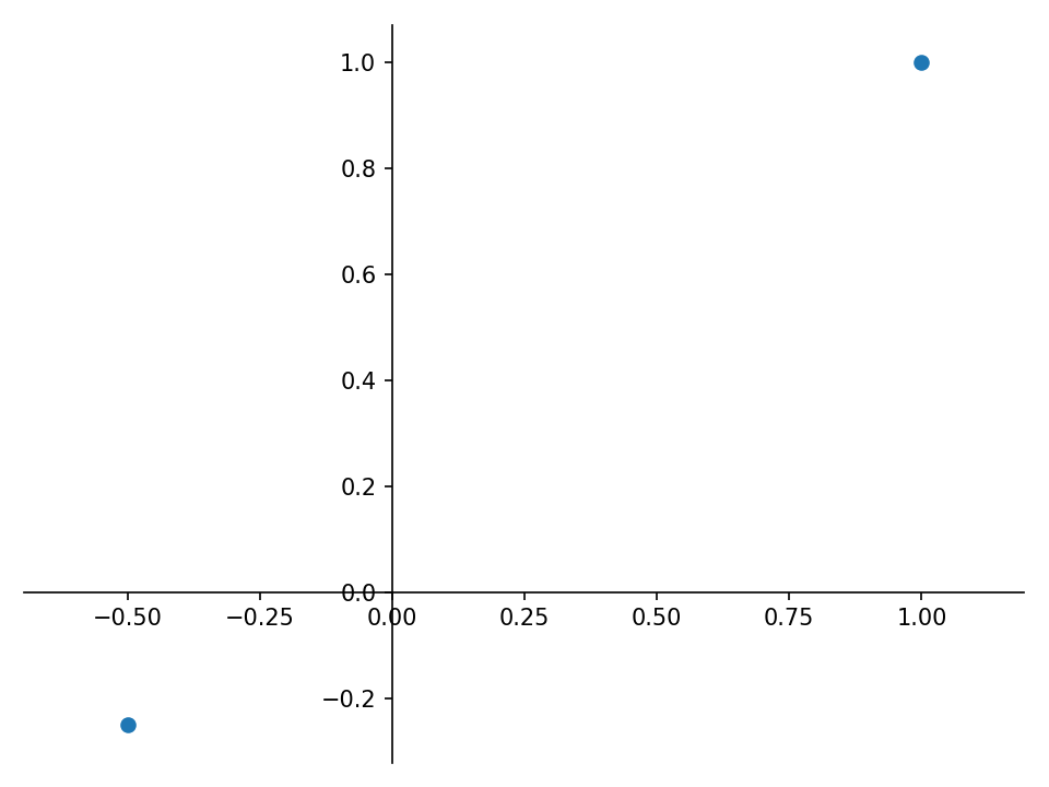
A complex number is, in essence, a "package deal" of two inseparable numbers. We can plot complex numbers in a Cartesian plane without any function in sight. Just consider the real part goes to X axis, and the imaginary part goes to Y axis:
If we plot a well-spread set of complex numbers whose absolute values are equal to 4, we end up with something that resembles a circle:
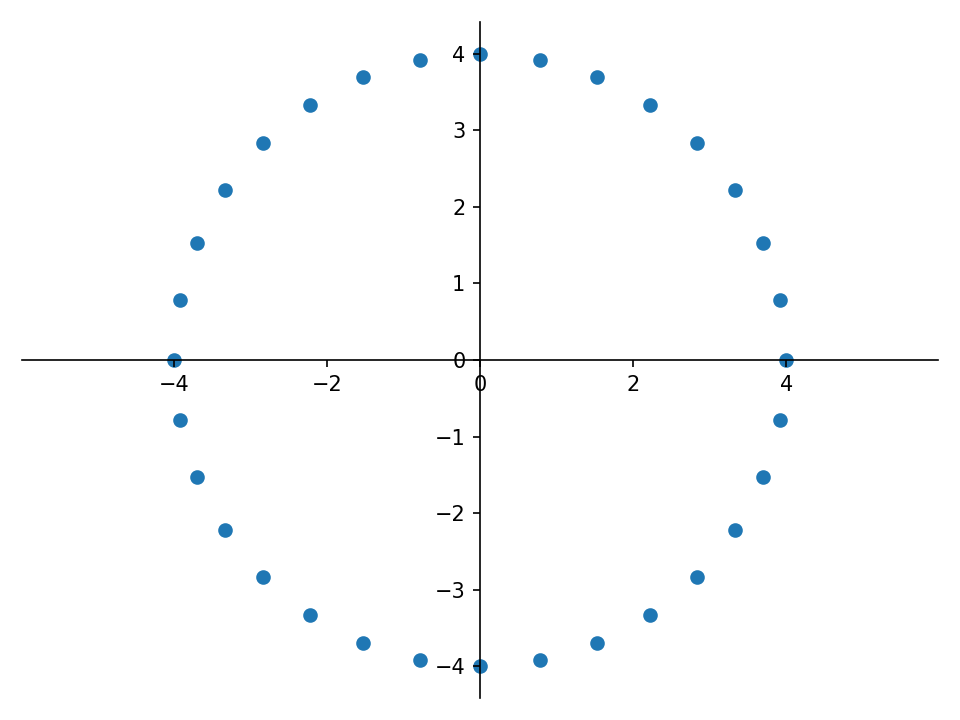
In the graph above, we can find numbers like 4, -4, 4i, -4i, 2√2+2√2i, etc. We can increase the density of the set until the points describe a smooth curve, a circle, which is closed and continuous:
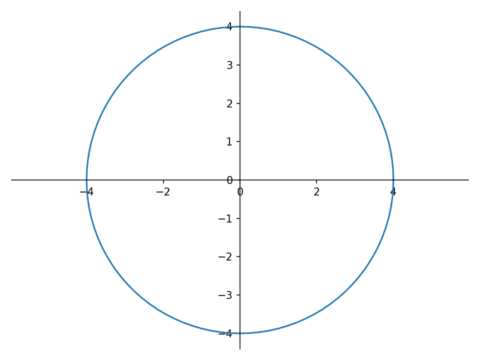
Note again, the graph above is not the graph of a function! It is just the graph of a bunch of complex numbers, that happen to describe a closed curve.
Now, if we apply a function on each number of this bunch, e.g. our quadratic polynomial, it is expected we get a new set of complex numbers, that will plot differently over the plane:
If we make both sets, domain and image, dense enough to describe a smooth curve,
So, this is the deal: a function that accepts complex numbers does not generate an ordinary chart. It generates a map or transform; it takes a curve and transforms into another. To see graphically what happens in a complex function, we need to compare the two curves.
Once you get this is the way it works in the realm of complex numbers, the FTA proof is easy to understand. In the next figures, we will use the polynomial
0,1x2 - 0,5x + 0.6
so the curves of x e f(x) have a similar scale for interesting ranges. It is the same polynomial as before, just multiplied by 0.1. The roots remain the same. As said before, we can always scale a polynomial without changing its essence.
First off, let's consider what happens when x is zero, or very small. In this case, all terms of the polynomial vanish, except the constant 0.6.
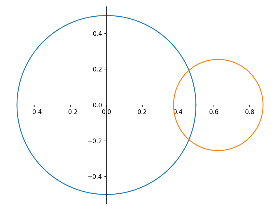
So, if we consider a set of complex values of x of small absolute value, that trace a small circle around the Cartesian origin, the image set generated by f(x) will trace a circle of the same size around the position (0.6, 0).
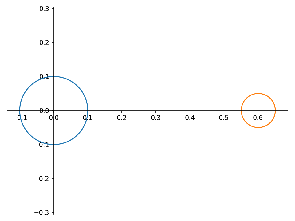
Obviously, x=0 is not a root of this polynomial, since f(0)=0.6. We can say we've found a root when we make the orange curve to cross exactly over the origin (0, 0). Also, note the Cartesian origin (0, 0) is outside the orange circle.
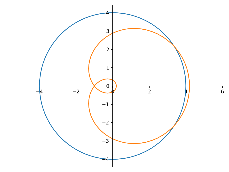
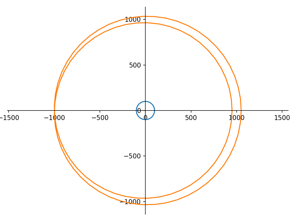
Great, we've seen what happens when x tends to zero. On the other hand, if we consider sets with evergrowing absolute values, f(x) also traces bigger and bigger curves:
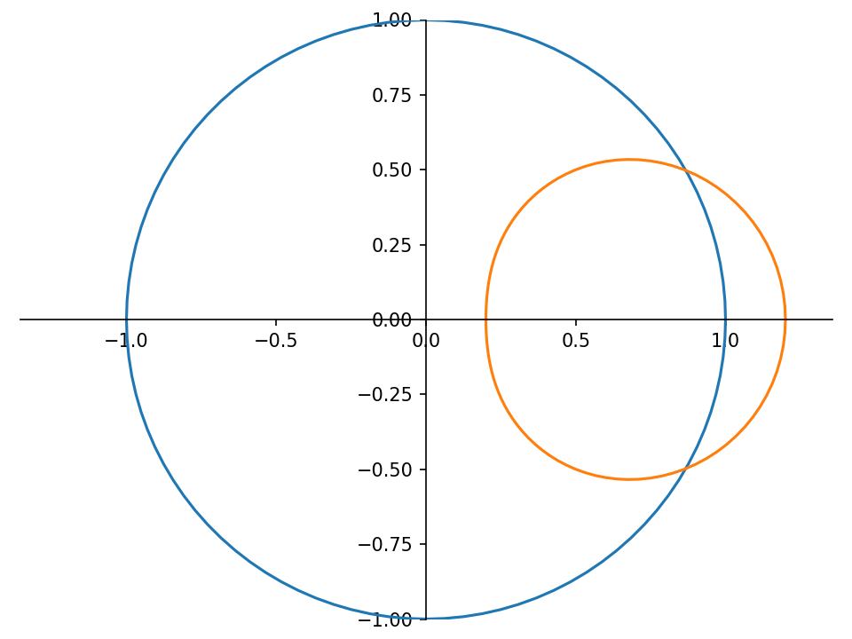
In the chart above, note the orange curve goes twice around. This is expected for any polynomial: if the degree were 3, the curve would go three times around, and so on.
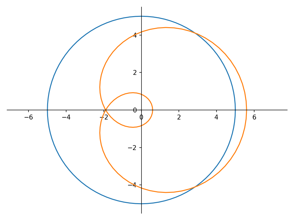
The orange curve still goes twice around, but the two loops are very near each other.
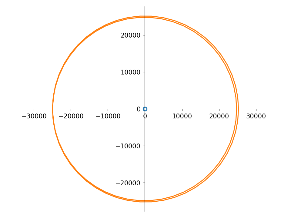
Now we can see that, for huge absolute values of x, the curve traced by f(x) looks more and more like a perfect circle with center at origin. It happens because the higher-degree term of the polynomial (x2) dominates the others and has overwhelming influence on the shape.
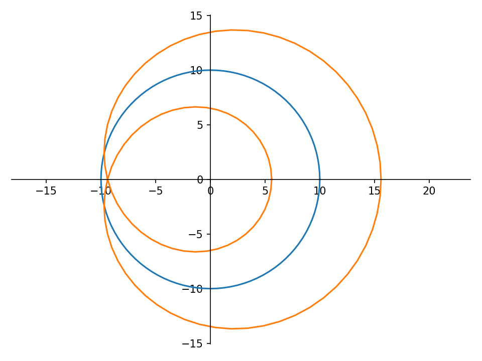
So, we can take for granted that, making |x| big enough, the curve of f(x) will be a big multi-looped circle. And the Cartesian origin (0, 0) will be inside this circle.
Now, the ace in the hole.
In the first case, when |x| is small, f(x) makes a very small circle that does not contain the Cartesian origin. In the second case, when |x| is big, f(x) makes a big circle that does contain the Cartesian origin.
Consider now that we start with |x|=0, and increase it slowly and continuously. At some moment, the Cartesian origin moves from outside to inside the orange curve.
Well, if we can tweak |x| in order to put the Cartesian origin inside, outside, far away or near from the orange curve, there must be a value of |x| in which the orange curve crosses exactly the coordinates (0, 0). That is, there is an x that makes f(x)=0.
We don't know exactly which values of x or |x| will do the trick (the FTA proofs are notoriously non-constructive) but we must accept that they exist.
Another, smoother version of the animation:
Most textbooks show only polynomials with integer or rational coefficients. But the FTA remains true even if the coefficients are irrational or complex numbers.
We learn at school that the complex roots of a polynomial equation always show up in conjugate pairs. For example, a cubic equation may have 1 or 3 real roots, while the quadratic equation may have 0 or 2 real roots.
The FTA has no relationship with this rule. Actually, the coefficients must be all real for the complex roots to be in conjugate pairs. Since all coefficients are symmetrical functions of the roots, the conjugate pairs allow the imaginary parts of the roots to cancel out inside the Viète formulas.
In general, the study of polynomials restricts their coefficients to the field of rationals (Q). Since their roots can be irrational and/or complex, the study of field extensions (i.e. find a field bigger than Q but smaller than R or C that still contains all roots) is the thing that makes the subject interesting, and motivated mathematicians like Lagrange, Ruffini, Abel and Galois.