A naïve lowpass FIR filter

Resuming from last post about the DFT audio filter, I mentioned that there were two other major methods do create a digital filter: FIR and IIR. This time I will demonstrate a FIR (Finite Impulse Response) filter.

First, we need to resort to some math. We have that operation called convolution, which can be understood as a kind of "graphical multiplication", controlled "blurring", or moving average.

Consider the following equation:

average stock index(day n) = 0.5 * index(day n) +
                             0.3 * index(day n-1) +
                             0.2 * index(day n-2)

This is a moving average of the stock market that takes three days into consideration, with different weights (0.5, 0.3, 0.2).

Figure 1: Graph with moving average

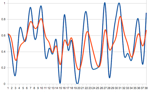
The graph of the moving average (red) against some simulated stock market movements (blue) shows clearly the smoothing effect. The red line follows the market but shortcuts peaks and valleys nicely.

In any given stock market, I may want to devise a "trend line", which is easier to see in a moving average curve than in the sizzly instantaneous market curve. Most technical analysis techniques are actually based on moving averages.

The red line can be understood as the convolution of two sequences: the blue line (which is, in theory, supposed to have no ends), and the list of weights, which has length three: [0.5, 0.3, 0.2].

Calculating a moving average line is not cheap. If there are three weights, three multiplications per point are needed. A 60-weights convolution over 5000 raw samples would demand 300k multiplications and 200k sums.

Moving averages make natural lowpass filters; and that's exactly what we are going to do soon, with audio.

There is a powerful relationship between time-domain and frequency-domain regarding convolutions. That is, what we are doing here is related to what we did in that article about Discrete Fourier Transform filtering.

Converting a signal from time domain to frequency domain has the power to "convert" a convolution to a simple multiplication, and vice-versa. This means that, if we can define a filter in frequency domain in terms of a multiplication, we can define the same filter in terms of a convolution in time domain.

Looking at DFT filter code, we have a section where we define a frequency "mask", which we multiply with actual song's spectral distribution, in order to make a bandpass filter:

mask = []
for f in range(0, FFT_LENGTH / 2 + 1):
    rampdown = 1.0
    if f > LOWPASS:
        rampdown = 0.0
    elif f < HIGHPASS:
        rampdown = 0.0
    mask.append(rampdown)

So, in principle, if we convert this frequency mask to a WAV file, and convolve it with our song, we achieve the same filtering result (save for rounding and quantization errors).

The WAV file generated from the filtering mask is not an audible wave, it is called the "impulse response". It is simply a list of weights, like we employed for the stock market's moving average, just longer.

We write it to a WAV file just to demonstrate that we don't need FFT anymore to filter the audio. The impulse response of a 3000Hz low-pass filter is something like this:

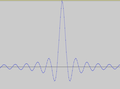
Figure 2: FIR filter impulse response

All we have to do is to convolve an actual audio with this impulse response, and the filtering will happen. That's the code:

#!/usr/bin/env python

import wave, struct, numpy
SAMPLE_RATE = 44100

original = wave.open("NubiaCantaDalva.wav", "r")
filter = wave.open("fir_filter.wav", "r")
filtered = wave.open("NubiaFilteredFIR.wav", "w")
filtered.setnchannels(1)
filtered.setsampwidth(2)
filtered.setframerate(SAMPLE_RATE)

n = original.getnframes()
original = struct.unpack('%dh' % n, original.readframes(n))
original = [s / 2.0**15 for s in original]

n = filter.getnframes()
filter = struct.unpack('%di' % n, filter.readframes(n))
filter = [s / 2.0**31 for s in filter]

'''
result = []
# original content is prepended with zeros to simplify convol. logic
original = [0 for i in range(0, len(filter)-1)] + original

for pos in range(len(filter)-1, len(original)):
    # convolution of original * filter
    # i.e. a weighted average of len(filter) past samples
    sample = 0
    for cpos in range(0, len(filter)):
        sample += original[pos - cpos] * filter[cpos]
    result.append(sample)
'''

result = numpy.convolve(original, filter)

result = [ sample * 2.0**15 for sample in result ]
filtered.writeframes(struct.pack('%dh' % len(result), *result))

Now, you are probably curious to hear the results. Here it is the original audio, and the filtered one.

(link to audio)

Note that there is a section of the program which is commented out. It implements convolution "manually" using two loops and basic arithmetic. This works perfectly well, and I left it (commented) in code just to make clear that convolution is matematically simple. The explicit implementation is terribly slow; using numpy.convolve() is much, much faster. Actually, this FIR filter is faster than the FFT version.

Of course, the FIR filter is fast but we need the impulse response calculated in advance. The following code generates this, and it needs to be run only once (or when you want to change the cut-off frequency of the filter):

#!/usr/bin/env python

LOWPASS = 3000 # Hz
SAMPLE_RATE = 44100 # Hz

import wave, struct, math
from numpy import fft
FFT_LENGTH = 512

NYQUIST_RATE = SAMPLE_RATE / 2.0
LOWPASS /= (NYQUIST_RATE / (FFT_LENGTH / 2.0))

# Builds filter mask. Note that this sharp-cut filter is BAD
mask = []
negatives = []
l = FFT_LENGTH / 2
for f in range(0, l+1):
    rampdown = 1.0
    if f > LOWPASS:
        rampdown = 0.0
    mask.append(rampdown)
    if f > 0 and f < l:
        negatives.append(rampdown)

negatives.reverse()
mask = mask + negatives

fir = wave.open("fir_filter.wav", "w")
fir.setnchannels(1)
fir.setsampwidth(4)
fir.setframerate(SAMPLE_RATE)

# Convert filter from frequency domain to time domain
impulse_response = fft.ifft(mask).real.tolist()

# swap left and right sides
left = impulse_response[0:FFT_LENGTH / 2]
right = impulse_response[FFT_LENGTH / 2:]
impulse_response = right + left

# write in a normal WAV file
impulse_response = [ sample * 2**31 for sample in impulse_response ]
fir.writeframes(struct.pack('%di' % len(impulse_response),
                                 *impulse_response))

Despite the simplicity, a FIR filter is not always faster than a FFT filter. The break-even is around 64 points; more than this, and FFT will be cheaper. Of course, implementations may change the break-even point: my 512-point FIR filter written in Python is still much faster than the FFT version, so it pays off to use FIR, in particular when the filter must operate in real-time.

The FIR filter is less powerful, in the sense that it cannot do every trick that FFT can. A frequency-domain filter that cannot be expressed in terms of a multiplication, cannot be converted to a time-domain convolution — that is, the filter is not realizable as a FIR filter. FIR is to FFT like a tin opener is to a Swiss-army knife.