 QAM modem: RX part
QAM modem: RX part
QAM modem: RX part
Following the discussion of a "QAM modem" written in Python, let's take a look into the reception (RX) code.
Decoding the QAM signal (reliably, at least) is much more complicated than generating it, and RX has much more code. Because of that, I will explain each section separately.
First, some boilerplate code:
#!/usr/bin/env python

import wave, struct, math, numpy, random

SAMPLE_RATE = 44100.0 # Hz
CARRIER = 1800.0 # Hz
BAUD_RATE = 360.0 # Hz
PHASES = 8
AMPLITUDES = 4
BITS_PER_SYMBOL = 5

# FIR lowpass filter. This time we calculated the coefficients
# directly, without resorting to FFT.
lowpass = []
CUTOFF = BAUD_RATE * 4
w = int(SAMPLE_RATE / CUTOFF)
R = (SAMPLE_RATE / 2.0 / CUTOFF)
for x in range(-w, w):
    if x == 0:
       y = 1
    else:
       y = math.sin(x * math.pi / R) / (x * math.pi / R)
    lowpass.append(y / R)

# Modem constellation (the same as TX side)
constellation = {}
invconstellation = {}
for p in range(0, PHASES):
    invconstellation[PHASES - p - 1] = {}
    for a in range(0, AMPLITUDES):
        s = p * AMPLITUDES + a
        constellation[s] = (PHASES - p - 1, a + 1)
        invconstellation[PHASES - p - 1][a + 1] = s

qam = wave.open("qam.wav", "r")
n = qam.getnframes()
qam = struct.unpack('%dh' % n, qam.readframes(n))
qam = [ sample / 32768.0 for sample in qam ]
Part of the code is borrowed from TX: modulation parameters, constellation generator etc. Those things would fit better in a separate module, but I was lazy to do it :) The constellation loop generates a reverse-map dictionary, since we are doing the inverse of TX (given amplitude and phase, give me the bits).
A new thing is the FIR filter generator. This time I did not use FFT to generate the coefficients; a closed-form expression was used instead. I am aware that this FIR filter is not the best possible (it ends abruptly at both sides), but served well enough for this toy.
# Demodulate in "real" and "imaginary" parts. The "real" part
# is the correlation with carrier. The "imaginary" part is the
# correlation with carrier offset 90 degrees. Having both values
# allows us to find QAM signal's phase.

real = []
imag = []
amplitude = []

# This proofs that we don't need to replicate the original carrier
# (at least, not in the same phase). Sometimes this random carrier
# phase makes the receiver to interpret training sequence as a
# character, but nothing serious.

t = int(random.random() * CARRIER)
# t = -1

# In the other hand, frequency must match carrier exactly; if we
# need to allow for frequency deviations, we must build a digital
# equivalent to PLL / VCO oscilator.

for sample in qam:
    t += 1
    angle = CARRIER * t * 2 * math.pi / SAMPLE_RATE
    real.append(sample * math.cos(angle))
    imag.append(sample * -math.sin(angle))
    amplitude.append(abs(sample))

del qam
UPDATE: the angle calculation is correct, even though 2 * math.pi * t / (SAMPLE_RATE / CARRIER) would look more like a textbook formula.
This was the "analog" part of the decoder. It is the most important, and the easiest to do, because trigonometry does so much for us.
From the analog AM modulation we learn that a demodulated signal has two components: the original information that we want to recover, and an undesirable demodulation "noise" around twice the carrier's frequency.
In QAM decoding, we found the "real" and "imaginary" parts, and both have the same noise. If you plot them in a graph, they won't make much sense. Both need to be filtered.
A bit of math to proof this point, that applies for AM and QAM as well. The original information f(t) is modulated by a cosine wave, so the transmitted signal is f(t).cos(t). Demodulation makes it f(t).cos(t).cos(t), which is equivalent to f(t).[1+cos(2t)], or f(t)+[f(t).cos(2t)].
In the last form we can see that demodulated signal is a sum of two parts: the decoded f(t) signal (that we want) and the same signal re-modulated at 2t (that we don't want).
Since we did a kind of AM modulation at TX, multiplying a digital signal by a sinusoid, we do the same at RX: multiply again by the sinusoid to get the original data. We don't know exactly the phase of QAM signal, and we don't need to. We just multiply by two local carriers, which are identical except by a 90 degress offset — math.cos() and math.sin().
Some readers were a bit puzzled: how we can extract two values (real and imag) from a single signal? Or how we can measure the phase of the signal just by multiplying them by cos(t) and -sin(t)?
This is indeed a fundamental difference between AM and QAM. In AM, the carrier never changes phase; only the variation of amplitude is employed, and only one data signal can be transmitted. In QAM, amplitude and phase are manipulated, so two data signals can travel together. Modulation methods like AM and PSK (Phase Shift Keying) are "degenerated" cases of QAM where phase or amplitude never changes, respectively.
Both modulation and demodulation use two orthogonal carriers of the same frequency cos(t) and -sin(t). In modulator, we manipulate the amplitude of each one to generate a QAM signal of any phase (and any amplitude). At demodulator, trigonometry allows us to reuse the same trick.
A bit of math can convince that the trick works at demodulation. Suppose that the original information is real=0, imag=-1. This renders a QAM signal equal to sin(t). At RX side this signal is multiplied by the quadrature carriers:
QAM = sin(t)
real = sin(t) * cos(t)  = sin(2t)
imag = sin(t) * -sin(t) = - 1 + cos(2t)

after filtering undesirable noise around frequency "2t":

real = 0
imag = -1
There are many ways to understand how QAM quadrature works. It may be seen as two simultaneous AM signals offset by 90 degrees, or it may be seen as a media capable of transmitting complex numbers, not just real ones. Or, as I said, that two physical quantities are manipulated (amplitude and phase) so we can transmit two pieces of data.
Of course, in the little mathematical exercise above, we assumed that that modulator and demodulator carriers have exactly the same phase, which is impossible to achieve. So in practice the QAM RX looks for phase changes.
Note this line of code, taken from the code snipped shown before:
t = int(random.random() * CARRIER)
Note that I set "t" with a random initial number, which means that carrier phase is random as well. This is a way to guarantee that local carrier will NOT be in phase with TX, and still the RX will be able to recover the data. So I can prove that looking for phase changes does work.
Incredible as it may seem, output of this demodulation is the X,Y position of symbol in modem constellation. The computed positions will be rotated, because local carrier is not in phase with original TX carrier, but since we have integrated the phase changes at TX, we just need to look for phase differences.
Finally, we "demodulated" amplitude in a separate channel, using abs(), just out of laziness, since we could obtain amplitude from real and imaginary parts.
It looks easy because we don't need to cope with frequency distortions. In practice, the local carrier would have to "tune" to the input signal, because AM demodulation depends on local carrier being exactly the same frequency as modulated signal. And all real-world transmission media distort frequency in some degree.
# Pass all signals through lowpass filter
real = numpy.convolve(real, lowpass)
imag = numpy.convolve(imag, lowpass)
amplitude = numpy.convolve(amplitude, lowpass)

# After lowpass filter, all three lists show something like
# a square wave, pretty much like the original bitstream.
# If you want to see the result of early detection phase,
# uncomment this:

# f = wave.open("teste.wav", "w")
# f.setnchannels(1)
# f.setsampwidth(2)
# f.setframerate(44100)
# bla = [ int(sample * 32767) for sample in imag ]
# f.writeframes(struct.pack('%dh' % len(bla), *bla))
As we said before, AM demodulation leaves a high-frequency residue in original data, so we pass our FIR filter in all signals (real, imaginary and amplitude). After this filtration, the signals will show themselves as quasi-square waves, like this:
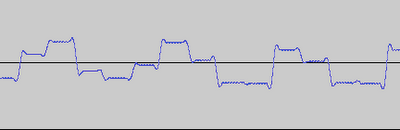
The filtered signal still has "rough edges" because, when the symbol changes, QAM signal suffers an abrupt change in phase and amplitude. This abrupt change throws noise on all frequencies (like a lightning generates all kinds of noise, from thunder to eletromagnetic interference). The low-pass filter can get rid of most, but not all of this noise.
This is a reason why the low-pass filter needs to be selective about frequencies above the baud rate. At first glance, a simpler and faster filter that removes the demodulation noise (centered at twice the carrier's frequency, so well above the baud rate) looks enough, but it would let more symbol-changing noise to pass.
Things might be a bit different in analog QAM. (Yes, there is analog QAM; it is used to transmit color information in analog TV.) In analog QAM, the information signal does not have a "baud rate" and there may be no abrupt changes, so the post-demodulation filtering may be easier.
It is also important to mention sampling rate at this point. The sampling rate needs to be high enough to contain the AM demodulation "noise". For example, if chosen carrier is 1800Hz, the demodulation noise will be around 3600Hz, so the sampling rate must be above 7200Hz. If the signal bandwidth (i.e. the baud rate) is significant, it must be added to 3600Hz.
Common sense says that, if we use a sampling rate a bit above the carrier rate, the demodulation noise falls above the Nyquist rate and it is simply left out. Unfortunately, a signal (or noise) above the Nyquist rate won't be magically filtered out; it will be distorted by frequency aliasing also known as "beating" or "folding". Trying to encode a 3500Hz signal using a sampling rate of 3600Hz (whose Nyquist rate of 1800Hz) will result in a 100Hz signal that is useless (for our purposes).
This means, that if you try to use a sample rate of 4000Hz to demodulate a QAM signal whose carrier is 1800Hz, the 3600Hz demodulation noise folds into the 400Hz range, mixing itself with the recovered message, destroying it.
So, in short, you need a pretty high sample rate and you need to employ some kind of low-pass filtering on recovered signal. There are no shortcuts.
Back to the demodulated signals graph, after filtering:

We have three square waves like this: real, imag, and amplitude. Now we have the mission of extracting the symbols out of them. First, we need to detect phase of symbols:
# Detect phase based on real and imaginary values

phase = []
wrap = 2.0 * math.pi * (PHASES - 0.5) / PHASES
for t in range(0, len(real)):
    # This converts (real, imag) to an angle
    angle = math.atan2(imag[t], real[t])
    if angle < 0:
        angle += 2 * math.pi
    # Move angle near to 2 pi to 0
    if angle > wrap:
        angle = 0.0
    phase.append(angle)
Since our constellation does not use complex numbers, the X,Y coordinates found by demodulator are not directly useful to search for the symbol, so we need to compute actual angles, which we do using atan2().
# Find maximum amplitude based on training whistle (1s), and
# measure how much our local carrier is out-of-phase in
# relationship to QAM signal

max_amplitude = 0.0
carrier_real = 0.0
carrier_imag = 0.0
for t in range(int(0.1 * SAMPLE_RATE), int(0.9 * SAMPLE_RATE)):
    max_amplitude += amplitude[t]
    carrier_real += real[t]
    carrier_imag += imag[t]

max_amplitude /= int(0.8 * SAMPLE_RATE)
carrier_real /= int(0.8 * SAMPLE_RATE)
carrier_imag /= int(0.8 * SAMPLE_RATE)

skew = math.atan2(carrier_imag, carrier_real)

print "Carrier phase difference: %d degrees" % (skew * 180 / math.pi)

del imag
del real
Here we analyze the "training" whistle sent by TX, in order to determine the amplitude range, as well as the phase difference between our carrier and TX carrier. We do this in a very lazy way here, and it would not be ok for a real-world modem.
Any real-world medium, be it wireless or wire or optics, does distort amplitude, phase and frequency, so it wouldn't work to estimate both at the beginning of session and leave it that way. Real-world modems use a PLL to generate local carrier, which adjusts itself all the time accordingly to input conditions.
# Normalize/quantify amplitude and phase to constellation steps
qsymbols = []
for t in range(0, len(phase)):
    p = phase[t]
    a = amplitude[t]
    a /= max_amplitude
    a = int(a * AMPLITUDES + 0.49) # adding 0.49 is a rounding trick

    # Compensate for local carrier phase difference
    # This ensures the best phase quantization (avoiding that
    # quantization edge is too near a constellation point)

    p += 2 * math.pi - skew
    p /= 2 * math.pi
    p = int(p * PHASES + 0.49) % PHASES

    qsymbols.append((p, a))

del phase
del amplitude
Here we take the "analog" phases and amplitudes, and quantize them into constellation. At this point we "unskew" the angles, so the quantified values map directly to our constellation.
The problem now is: we have thousands of samples that contain just a handful of symbols. We need to detect how many symbols are there — and where.
# Try to detect edges between symbols

edge = []
settle_time = int(SAMPLE_RATE / BAUD_RATE / 8)
settle_timer = -1
in_symbol = 0
first_symbol = 0
last_a = last_p = 0
for t in range(0, len(qsymbols)):
    s = 0
    p, a = qsymbols[t]
    if in_symbol > 0:
        # we presume we are flying over a valid symbol
        in_symbol -= 1
    elif a != last_a or p != last_p:
        # change detected, look for stabilization in future
        settle_timer = settle_time
    elif settle_timer > 0:
        # one sample closer a good symbol
        settle_timer -= 1
    elif settle_timer == 0:
        # signal settled for (settle_time) samples;
        # take the current signal as a valid symbol
        settle_timer = -1
        in_symbol = int(0.85 * SAMPLE_RATE / BAUD_RATE)
        if t > 0.5 * SAMPLE_RATE:
            # make sure we are not at the beginning
            s = 1
            if not first_symbol:
                first_symbol = t
    edge.append(s)
    last_p = p
    last_a = a
At this section, we count on the fact that most symbols show a distinctive "edge" between them. We annotate the points where this edge is present, for further reference.
Note that this step did not find all symbols, because the message may have repeated symbols with phase 0, without a distinct edge between them. This is a direct result of poor constellation choice; it would have been better to avoid phase-0 points, so we would find all symbols by looking for edges.
# Find symbols based on edges and known baud rate

symbols = []
expected_next_symbol = SAMPLE_RATE / BAUD_RATE
lost = 0

for t in range(first_symbol - int(SAMPLE_RATE * 0.1), len(qsymbols)):
    p, a = qsymbols[t]
    s = edge[t]

    if s:
        # amplitude/phase edge, strong hint for symbol
        lost = 0
        symbols.append([p, a])
    else:
        lost += 1

    if lost > expected_next_symbol * 1.5:
        # no edge yet, take this as a non-transition signal
        lost -= expected_next_symbol
        symbols.append([p, a])

del qsymbols
del edge
Here we finally detect the handful of symbols we are interested in, and we can throw out the enormous time-domain lists.
The strategy of symbol detector is simple. Every detected edge is a new symbol for sure. But, if no edge was found after some time (baud rate + 50% tolerance), we blindly assume that we have a repeated symbol there.
Even if TX and RX baud rates were a bit different, this strategy would be robust, because most symbols do have an edge between them, so the algorithm can keep the clock always syncronized.
print "%d symbols found" % len(symbols)

# Differentiate phase (because we had integrated it at transmitter)

last_phase = 0
for t in range(0, len(symbols)):
    p = symbols[t][0]
    symbols[t][0] = (p - last_phase + PHASES) % PHASES
    last_phase = p
In TX we had integrated (summed up) the phase offsets, so now we have to do the opposite operation.
# Translate constellation points into bit sequences

bitgroups = []
for t in range(0, len(symbols)):
    p, a = symbols[t]
    try:
        bitgroups.append(invconstellation[p][a])
    except KeyError:
        print "Bad symbol:", p, a, ", ignored"

# Translate bit groups into individual bits

bits = []
for bitgroup in bitgroups:
    for bit in range(0, BITS_PER_SYMBOL):
        bits.append((bitgroup >> (BITS_PER_SYMBOL - bit - 1)) % 2)
Symbol characteristics are traded for bit sequences, and finally we can see the actual bits we were looking for. The demodulation is done, but now we have to recover bytes from bits, like an RS-232 interface would do.
# Find bytes based on start and stop bits. This will make you feel
# like a poor RS-232 port :)

t = 0
state = 0
byte = []
bytes = []
while t < len(bits):
    bit = bits[t]
    if state == 0:
        # did not find start bit
        if not bit:
            # just found start bit
            state = 1
    elif state == 1:
        # found start bit, accumulating a byte
        if len(byte) < 8:
            byte.append(bit)
        else:
            # byte complete, test stop bit
            if bit:
                # stop bit is there
                bytes.append(byte)
            else:
                # oops, stop bit not there, we were cheated!
                # backtrack to the point fake start bit was 'found'
                t -= 8
            byte = []
            state = 0
    t += 1

# Make a string from the bytes

msg = ""
print "Bytes:",
for byte in bytes:
    value = 0
    for bit in range(0, 8):
        value += byte[bit] << (8 - bit - 1)
    msg += chr(value)
    print value,

print
print msg
The serial-to-bytes loop looks for start bits (zeros) and stop bits (ones). Once it finds a bit sequence that satisfies these conditions, it cuts a byte. If either the start or stop bit is missing, it keeps reading bits until synchronization is again found.
Amazingly, this thing works. The improvements I can imagine for this Python modem are:
1) Take a closer look at the FIR filter, choosing the best cutoff frequency and avoid abrupt ends.
2) Choose a better constellation, without 0-phase points, and use complex numbers.
3) Generate the RX local carrier using a PLL (phase-locked loop), so it can "follow" frequency and phase distortions.
4) Measure amplitude range continually using AGC (automatic gain control).
5) Add a bit randomizer.