 Radio scanning with Python
Radio scanning with Python
Radio scanning with Python
In this article, we describe the innards of a "radio scanner" and automatic recorder, developed with Python language and works with an ordinary SDR dongle.
It is not a true radio scanner in the sense that it does not sweep the band; it monitors a static (but relatively wide) band. A true scanner can be developed using our program as a starting point.
Our program is a pretty interesting toy, as-is (everybody likes to "eavesdrop" and listen to "private" conversations), as a good example of a couple DSP concepts, and as a stepping stone to tinker and develop any number of improvements.
First off, here is a demonstration of what it can do:
In this example session, the program listens many GMRS channels. GMRS are used by two-way radios like the well-known Motorola Talkabout. Audio is recorded only when a "good" signal is detected.
In the GitHub repository, there are many scripts that leverage the same base program nfm.py to scan channels in VHF range, UHF, GMRS, aviation and ATIS. The program is named "nfm" meaning "narrow FM" but it can decode AM as well.
Note: merely listening to analog, non-encrypted radio signals is legal in most jurisdictions. There are some exceptions e.g. Germany. Publishing the contents (transcriptions or the raw audio) is probably illegal in most jurisdictions, in particular when it violates someone's privacity in any way.
FM broadcast stations occupy a wide band, 200kHz each, in order to achieve high-fidelity sound with a relatively old analog technology. In the realm of two-way voice communications (aviation, police, public services, FM amateur radio), intelligible voice is enough. Each channel occupies a very narrow band, around 10kHz.
In this realm, the most common analog modulation is FM, even though aviation uses AM. The general trend is to migrate to digital modes (DMR, P25) since they use even less bandwidth and can be encrypted. The regulatory agencies tend to insist that new licenses are digital-only, to squeeze as many users as possible in the crowded sub-GHz bands.
It is also noteworthy these two-way radio bands are "channelized", that is, each channel has a well-defined frequency and bandwidth. In amateur radio, there are non-channelized bands e.g. Morse and AM/SSB can be transmitted in any frequency, as long as they are within the designated band. The receiver must search for a signal and fine-tune it for perfect demodulation. (Of course hams have their conventions about frequencies and timetables, to find each other more easily.)
For professional uses, fixed channels are much more practical. Hams also use FM voice channels, more than any other mode. For technical reasons, analog AM and FM modulations work fine with fixed channels, while SSB does not, since it always takes manual fine-tuning.
As mentioned in the article about broadcast FM, an RTL-SDR dongle cannot filter a very narrow band by itself. The workaround is to capture a wider band and filter the narrower band by software. On the other hand, two-way radio channels are often clustered, so we can eavesdrop many of them with a single dongle.
The script below was used in the demonstration video:
BW=250000
CHANNEL_BW=12500
FREQS="462562500 462587500 462612500 462637500 462662500 462687500 \
	462712500 462550000 462575000 462600000 462625000 462650000 \
	462675000 462700000 462725000"
STEP=2500

# Determine center automatically
s=0
n=0
for f in $FREQS; do
	s=$(($s + $f))
	n=$(($n + 1))
done
CENTR=$(($s / $n))
CENTR=$(($CENTR / $STEP))
CENTR=$(($CENTR * $STEP))

rtl_sdr -f $CENTR -g 30 -s $BW - | \
	./nfm.py $CENTR $BW $STEP $CHANNEL_BW $FREQS . -a $*
The BW variable is the total bandwidth being monitored. This bandwidth must be compatible with the SDR dongle. (For RTL-SDR and it clones, that would be 200-300k or 900k-2800k.) The raw bandwidth must be ~20% bigger than the band of interest. It must also be a multiple of 25000, for internal reasons of our program.
The CHANNEL_BW variable is the bandwidth of one channel. For analog Talkabout, it is 12.5kHz.
The FREQS variable is the list of channel frequencies we want to record. The more channels, the more CPU the program will demand. If there are too many, the program won't be able to work real-time anymore. The suggestion is to start with every few channels and increase the list steadily, checking if CPU usage is below 100% in each core.
Moreover, the difference between the highest and lowest channel must "fit" within BW. This difference must be around 20% smaller than BW, since RTL-SDR filtering is not perfect and distorts the extremes of the bandwidth.
The STEP variable is a "common denominator". All other variables must be multiples of STEP, and STEP must divide 25000. This allows for many optimizations within our program. STEP is chosen to match CHANNEL_BW, since CHANNEL_BW is the invariant.
The CENTR variable is calculated automatically in our script. This is the central frequency captured by RTL-SDR. (It would have been more elegant to calculate this value within Python, but the vice of overusing shell script is difficult to lose.)
Two parameters passed to rtl_sdr may need some tweaking: the gain (-g) and the frequency correction (-p). For automated recording, I prefer to use a fixed gain; we will come back to this in the Squelch section. The frequency correction is negligible if you have a genuine RTL-SDR dongle. It drifts 1 or 2ppm at the most. "Generic" dongles can drift 50-70ppm as they warm up.
Now, let's see how the proper program nfm.py, works. Here is where the magic actually happens.
The audio detection is carried out as follows:
We use the NumPy library extensively, which allows us to achieve a decent performance without resorting to Cython or any other lower-level technique.
The first block is nothing new. The I/Q samples delivered by RTL-SDR are converted to a list of complex numbers.
# Convert to complex numbers
iqdata = numpy.frombuffer(data, dtype=numpy.uint8)
iqdata = iqdata - 127.5
iqdata = iqdata / 128.0
iqdata = iqdata.view(complex)

# Forward I/Q samples to all channels
for k, d in demodulators.items():
	d.ingest(iqdata)
We use threads in channel demodulators in order to put the multiple CPU cores into good use. The dreaded "GIL" is not a problem here since the heavy lifting happens within NumPy, and NumPy releases the GIL when it can.
The basic principle of complex demodulation is the same as ordinary demodulation: to move the channel of interest to the vicinity of frequency zero, so it becomes baseband again, as the original signal (audio).
# Get a cosine table in correct phase
carrier = self.carrier_table[self.if_phase:self.if_phase \
				+ len(iqsamples)]
# Advance phase
self.if_phase = (self.if_phase + len(iqsamples)) % self.if_period
# Demodulate
ifsamples = iqsamples * carrier
The last row is a product of two lists, implemented by NumPy and therefore fast.
One thing is, "carrier" is not a list of real numbers. It is a sequence of complex numbers. Moreover, we precompute it when the program starts, and we always reuse the same list:
self.if_freq = freq - CENTER
self.carrier_table = \
	[ cmath.exp((0-1j) * tau * t * (self.if_freq / INPUT_RATE)) \
		for t in range(0, INGEST_SIZE * 2) ]
The formula with cmath.exp() looks intimidating, but all it does is to calculate two quadrature carriers at once, one is stored in the real part of each sample, the other is stowed in the imaginary part.
For the precomputing optimization to be possible, the carrier period must fit in an integer number of samples, and this is one reason why all bands and frequencies must be multiples of STEP.
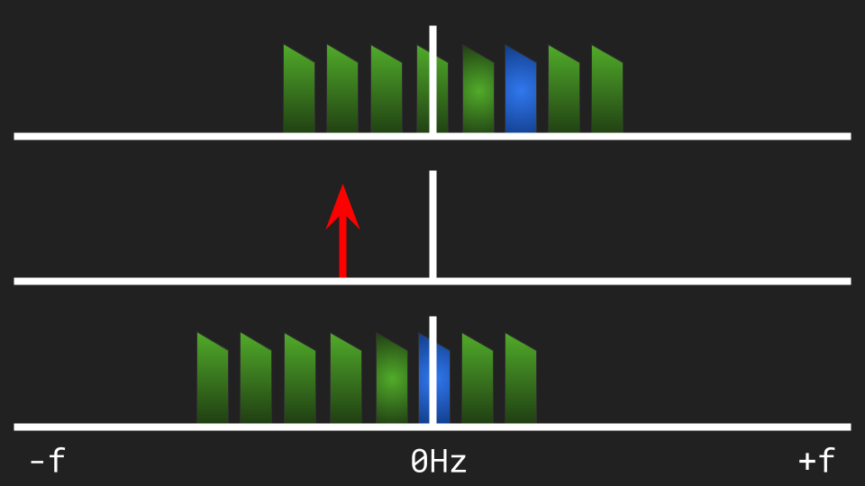
The I/Q signal from RTL-SDR is complex as well. The complex demodulation of a complex signal has a huge upside: it merely shifts the signal in the spectrum, and does not create any additional copies of the signal:
In the AM modulation, we always had to worry about the additional copies after modulation or demodulation, getting rid of them with filters, or using more advanced techniques.
Why complex modulation is different from AM modulation? There are two reasons that stem from the same fundament.
The first reason: a purely real carrier can be modeled as the sum of two complex carriers "rotating" in opposite directions i.e. one with positive frequency, another with negative frequency. The spectrum of a real carrier is symmetric around zero.
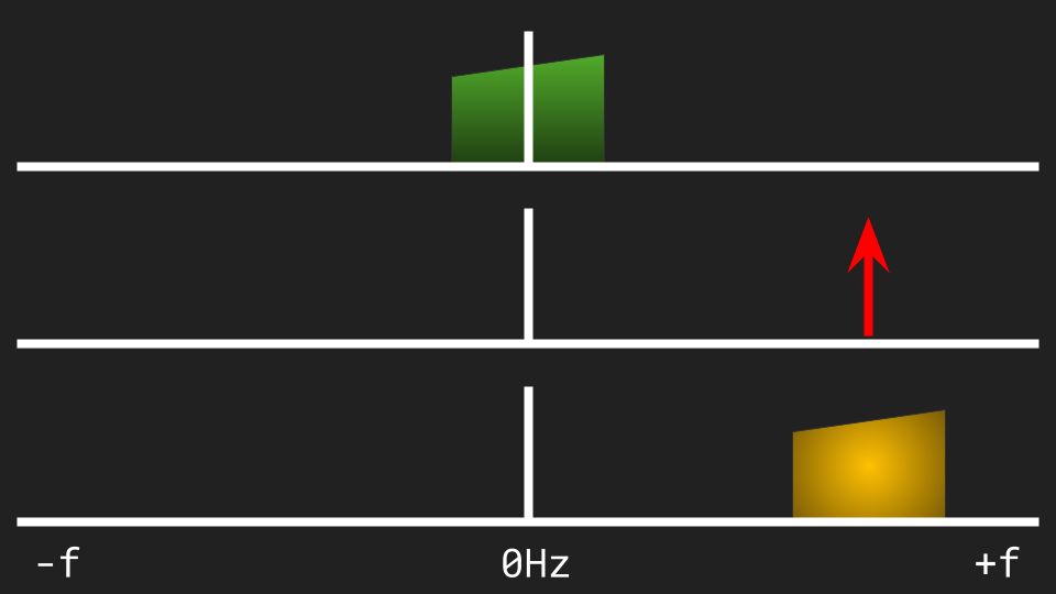
The modulation of a complex signal by a real carrier yields two copies, one of them at the negative side of the spectrum:
The second reason is, every purely real signal has symmetrical spectrum (*). That is, the spectrum at negative frequencies is a perfect mirror of the positive side. From the spectral point of view, such a signal already has two copies, but one of them is "hidden", since we don't think in terms of negative frequencies in the real world.
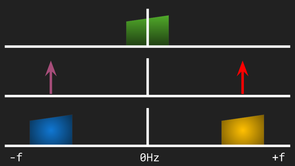
When a real signal is modulated by a complex carrier, the two mirror copies are shifted together:
We can argue that modulating a real signal with a real carrier generates nothing less than four copies of the signal:
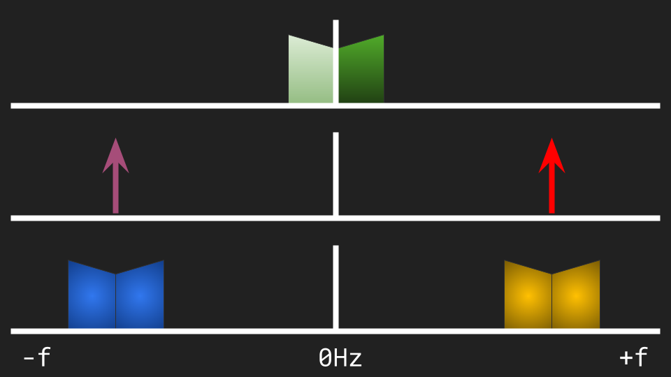
Since the result is symmetric, the modulated signal is purely real. This was expected, since the constituents were both real. (Only real signals can materialize themselves in the real world, be it in the form of radio waves or audio. Every modulation technique must take care the final output is realizable.)
Another "magical" trait of complex signals is the capability of holding different contents at positive and negative sides of the spectrum. Positive or negative carriers can be used to shift the spectrum to the right or to the left, respectively.
If the signal contains several channels or sub-bands, the first step to isolate the channel of interest is shifting it to baseband.
(*) A real signal has symmetric or "even" spectrum for the amplitude, and anti-symmetric or "odd" spectrum for the phase.
At this point, the channel we want to listen is the baseband, but the other channels are still present in the signal. We remove them with a lowpass filter.
self.if_filter = filters.low_pass(INPUT_RATE, IF_BANDWIDTH / 2, 48)
...
ifsamples = self.if_filter.feed(ifsamples)
We use our own filter implementation. It is a vanilla FIR filter, based on NumPy convolutions that are fast.
The filter works with real signals as well as with complex signals. It removes all frequencies (positive or negative) whose absolute value is higher than the cutoff.
At this point we can downsample the signal to optimize the further processing of the remaining channel.
self.if_decimator = filters.decimator(INPUT_RATE // IF_RATE)
...
ifsamples = self.if_decimator.feed(ifsamples)
There are two basic methods of converting the sampling rate of a digital signal: downsample by decimation, and upsample by stuffing. Either can do integer conversions only (1:2, 2:1, 1:3, 3:1, etc.) If a rational conversion si necessary (3:2, 3:4, etc.) we use a combination of upsampling and downsampling.
To upsample e.g. from 100 to 300 samples/s, we insert two zero samples after each original sample. This will insert high-frequency noise, which can be removed by a lowpass filter with cutoff 50. (The Nyquist Theorem says that a digitally-sampled signal of 100 can carry frequencies up to 50.)
To downsample it from 300 to 100, we keep 1 every 3 samples, discarding the other 2. This is called decimation, and the result would be distorted by the aliasing of high frequencies. To avoid this, we apply the lowpass filter before the decimation.
We had already filtered the unwanted channels, so the decimation can be carried out right away.
The intermediate sampling rate IF_RATE is 25000, and this number is not configurable in the present version of the program. Therefore, the sampling rate coming from RTL-SDR (the BW variable of the script) must be a multiple of 25000.
The FM audio detection is well described in this article. The basic idea is to translate phase shifts to audio samples, without regards to the absolute values.
The AM detection is exactly the opposite: the absolute values of the complex samples are translated to audio, regardless of phase.
if am:
	output_raw = numpy.absolute(ifsamples)[1:]
	output_raw *= 0.25 / strength
else:
	angles = numpy.angle(ifsamples)
	rotations = numpy.ediff1d(angles)
	rotations = (rotations + numpy.pi) % (2 * numpy.pi) - numpy.pi
	output_raw = numpy.multiply(rotations, DEVIATION_X_SIGNAL)
In AM, the audio volume is scaled proportionally to the added carrier, that shows up in demodulated audio as a big DC bias. (See the page about AM modulation to learn why there is an added carrier.)
The output of this stage is an audio signal, no longer complex, but purely real. As we said before, only a real signal can have real-world meaning — sound waves in this case.
In two-way radios, squelch cuts off the speaker when the reception level is too low. In our program, we implement something similar, so audio is recorded in WAV files only when there seems to be a signal.
if use_autocorrelation:
	vote = self.vote_by_autocorrelation(output_raw)
else:
	vote = self.vote_by_dbfs(dbfs)
Most radios implement squelch based on radio signal strength. We also implement this technique, it is activated when the -a parameter is omitted. This technique works when the signal/noise ratio is very high, which is the case of narrowband modes.
strength = numpy.sum(numpy.absolute(ifsamples)) / len(ifsamples)
dbfs = 20 * math.log10(strength)
...
def vote_by_dbfs(self, dbfs):
	vote = -1
	if dbfs > (self.dbfs_off + THRESHOLD_SNR):
		vote = +1
	if not self.is_recording and vote < 0:
		# Use sample to find background noise level
		if dbfs < self.dbfs_off:
			self.dbfs_off = 0.05 * dbfs \
				+ 0.95 * self.dbfs_off
		else:
			self.dbfs_off = 0.005 * dbfs \
				+ 0.995 * self.dbfs_off
	return vote
As can be seen above, we use a moving average of signal strength, and we also try to detect the background noise level automatically.
In this mode, rtl_sdr must operate with fixed gain (parameter -g with positive value). Otherwise, RTL-SDR would amplify the background noise when there is no signal, making I/Q signal strengh look the same with or without reception.
This squelch technique works well for AM signals, where the added carrier is a huge canary, even if audio is muted.
The other squelch method, that works very well with FM signals, is the autocorrelation.
def vote_by_autocorrelation(self, output_raw):
	ac_r = numpy.abs(numpy.correlate(output_raw, output_raw, \
			'same'))
	ac_metric = numpy.sum(ac_r) / numpy.max(ac_r) \
		/ len(output_raw)

	if self.ac_avg is None:
		self.ac_avg = ac_metric
	else:
		self.ac_avg = 0.2 * ac_metric + 0.8 * self.ac_avg

	vote = -1
	if ac_metric > THRESHOLD_AC:
		vote = +1
	return vote
We also smooth the autocorrelation value by a moving average. This technique deserves a longer explanation.
Correlation is a measure of similarity between two signals. A typical way of calculating it is to multiply the signals, sample by sample, and sum all products. The bigger the absolute value, the most similar are the signals.
For example, if we multiply cos(x) by sin(x), sample by sample, the sum of products will be zero, since these signals are 100% orthogonal, and they can even coexist in the same medium without interference.
On the other hand, correlating cos(x) by a shifted version of sin(x) will yield non-zero results. The extreme case is to correlate cos(x) with cos(x), that yields the maximum value (a signal is obviously very similar to a non-shifted version of itself!).
In the cos(x)/sin(x) example, we could see the correlation depends on phase shift. So, to effectively calculate a correlation, we must shift one signal to all possible offsets. If we are going to correlate two blocks of 100 samples, we have 299 unique offsets to test. What we want is to calculate the convolution of those two signals. The area of the convolution is the phase-invariant correlation.
Autocorrelation is simply to calculate the correlation of the signal with itself. If the signal possesses any internal pattern, the autocorrelation should be big. A signal carrying voice or date will show regular patterns along the time, some periodic trait, it will look like a phase-shifted version of itself.
On the other hand, if the signal is just white noise, every little piece is completely different from any other. The signal does not look similar to any shifted version of itself. The autocorrelation should tend to zero, and we interpret this as no reception.
A remaining question: why correlation does not work so well for AM? Possibly because AM is sensitive to QRM, that is, artificial noise sources. QRM looks "regular" and fools the algorithm. FM is notoriously resistant to QRM; an out-of-tune FM radio listens only QRN, the natural, thermal background noise.
The sampling rate is again reduced from 25000 to 12500. As said before, the signal must be filtered before decimation. In this stage, we use a cutoff of 4000Hz, since the typical two-way radio does not go beyond 3400Hz.
output_raw = self.audio_filter.feed(output_raw)
output = self.audio_decimator.feed(output_raw)
output = self.dc_filter.feed(output)
output = numpy.clip(output, -0.999, +0.999)
Also, we remove the DC Bias using a highpass filter. This bias shows as a constant value added to audio samples — mostly in AM signals, in which the DC Bias comes from the added carrier.
If the squelch algorithm finds that we are getting reception, the audio samples are written in a WAV file. Each channel lands in a different file.
if self.insert_timestamp:
	output = numpy.concatenate((self.gen_timestamp(output), \
					output))
	self.insert_timestamp = False

bits = struct.pack('<%dh' % len(output), *output)
if not self.wav:
	self.create_wav()
self.wav.writeframes(bits)
A WAV file will contain any number of recorded fragments. In case we need to separate them afterwards, each fragment has a short, inaudible preamble of pseudo-audio samples. This preamble embeds a timestamp.